You can draw 3D plot in cylindrical coordinate system using nf3d and plot3d1 functions.
You must transform from cylindrical coordinate system to cartesian coordinate system.
But It’s easy because what you have to do is only to use the conventional description as highlighted bellow.

clf(); //To clear the previous plot
xset('colormap', pinkcolormap(32));
funcprot(0); //nothing special is done when a function is redefined
function [z] = f(r, t)
    z = r'^2 * sin(2*t) / 2;
endfunction
r = linspace(0, 1, 20);
t = linspace(0, 2*%pi, 20);
x = r' * cos(t);
y = r' * sin(t);
z = f(r, t);
[xf, yf, zf] = nf3d(x', y', z');
plot3d1(xf, yf, zf, theta = 300, alpha = 60, leg = "@@", flag = [1 6 4]);





















You can draw a part of 3D plot by changing parameter's ranges.

clf(); //To clear the previous plot
xset('colormap', pinkcolormap(32));
funcprot(0); //nothing special is done when a function is redefined
function [z] = f(r, t)
    z = r'^2 * sin(2*t) / 2;
endfunction
r = linspace(.5, 1, 20);
t = linspace(0, 3*%pi/2, 20);
x = r' * cos(t);
y = r' * sin(t);
z = f(r, t);
[xf, yf, zf] = nf3d(x', y', z');
plot3d1(xf, yf, zf, theta = 300, alpha = 60, leg = "@@", flag = [1 6 4]);





















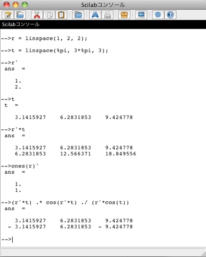
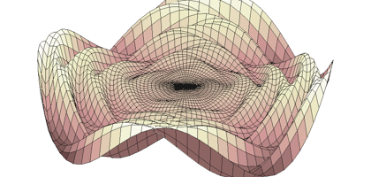
You must represent x to z by the matrix, which is column vector r' by row vector t, using ones() function and .* operator. ones() returns a matrix made of ones. A .* B represent that A elementwisely multiplied by B. See following example.

clf(); //To clear the previous plot
xset('colormap', pinkcolormap(32));
funcprot(0); //nothing special is done when a function is redefined
function [z] = f(r, t)
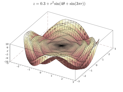
    z = 0.3 + (r'^2*ones(t)) .* sin(4*ones(r)'*t + sin(3*%pi*r)'*ones(t));
endfunction
r = linspace(0, 3, 40);
t = linspace(0, 2*%pi, 80);
x = r' * cos(t);
y = r' * sin(t);
z = f(r, t);
[xf, yf, zf] = nf3d(x', y', z');
plot3d1(xf, yf, zf, theta = 300, alpha = 8, leg = "@@", flag = [1 2 4]);
xtitle('$z=0.3+r^{2}\sin(4\theta+\sin(3\pi r))$');
a = gca(); //get the current axes
a.title.font_size = 4;



















The following is the example of vector and matrix operatings in Scilab.





























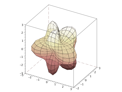
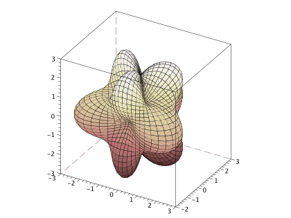
You can draw 3D plot in spherical coordinate system in the same way.
Highlighted bellow is the conventional description.

clf(); //To clear the previous plot
xset('colormap', pinkcolormap(32));
funcprot(0); //nothing special is done when a function is redefined
deff('r = f(t, p)', 'r = 2 + sin(3*p) * sin(3*t)')
function [r] = f(t, p)
    r = 2 + sin(3*t)' * sin(3*p);
endfunction
t = linspace(0, %pi, 20);
p = linspace(0, 2*%pi, 30);
r = f(t, p);
x = r .* (sin(t)' * cos(p));
y = r .* (sin(t)' * sin(p));
z = r .* (cos(t)' * ones(p));
[xf, yf, zf] = nf3d(x', y', z');
plot3d1(xf, yf, zf, theta = 300, alpha = 60, leg = "@@", flag = [1 6 4]);





















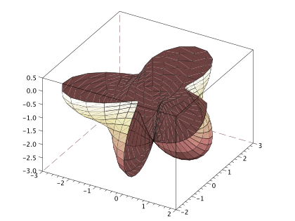
You can draw a part of 3D plot by changing parameter's ranges.

clf(); //To clear the previous plot
xset('colormap', pinkcolormap(32));
funcprot(0); //nothing special is done when a function is redefined
function [r] = f(t, p)
    r = 2 + sin(3*t)' * sin(3*p);
endfunction
t = linspace(%pi/2, %pi, 20);
p = linspace(0, 3*%pi/2, 30);
r = f(t, p);
x = r .* (sin(t)' * cos(p));
y = r .* (sin(t)' * sin(p));
z = r .* (cos(t)' * ones(p));
[xf, yf, zf] = nf3d(x', y', z');
plot3d1(xf, yf, zf, theta = 300, alpha = 60, leg = "@@", flag = [1 6 4]);





















You can increase the number of plot points for drawing more details.

clf(); //To clear the previous plot
xset('colormap', pinkcolormap(32));
funcprot(0); //nothing special is done when a function is redefined
function [r] = f(t, p)
    r = 2 + sin(3*t)' * sin(3*p);
endfunction
t = linspace(0, %pi, 40);
p = linspace(0, 2*%pi, 60);
r = f(t, p);
x = r .* (sin(t)' * cos(p));
y = r .* (sin(t)' * sin(p));
z = r .* (cos(t)' * ones(p));
[xf, yf, zf] = nf3d(x', y', z');
plot3d1(xf, yf, zf, theta = 300, alpha = 60, leg = "@@", flag = [1 6 4]);





















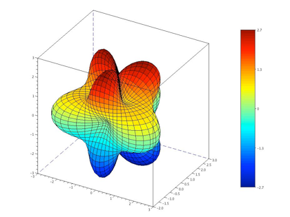
You can add the color bar by using colorbar function.
When you use colorbar function, you’ll be failed in outputting a postscript image as EPS format,
although Scilab’s postscript images are not beautiful usually.

clf(); //To clear the previous plot
xset('colormap', jetcolormap(64));
funcprot(0); //nothing special is done when a function is redefined
function [r] = f(t, p)
    r = 2 + sin(3*t)' * sin(3*p);
endfunction
t = linspace(0, %pi, 40);
p = linspace(0, 2*%pi, 60);
r = f(t, p);
x = r .* (sin(t)' * cos(p));
y = r .* (sin(t)' * sin(p));
z = r .* (cos(t)' * ones(p));
[xf, yf, zf] = nf3d(x', y', z');
plot3d1(xf, yf, zf, theta = 300, alpha = 60, leg = "@@", flag = [1 6 4]);
colorbar(min(z), max(z));





















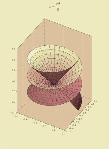
The following is an another sample of cylindrical coordinate plot.
You can add a title in TEX description and use many options as highlighted bellow.

clf(); //To clear the previous plot
xset('colormap', pinkcolormap(32));
funcprot(0); //nothing special is done when a function is redefined
function [z] = f(r, t)
    z = r' * t / 8;
endfunction
r = linspace(0, 1, 10);
t = linspace(-2*%pi, 4*%pi, 100);
x = r' * cos(t);
y = r' * sin(t);
z = f(r, t);
[xf, yf, zf] = nf3d(x', y', z');
plot3d1(xf, yf, zf, theta = 300, alpha = 50, leg = "@@", flag = [1 6 4]);
xtitle('$z=\frac{r\theta}{8}$');
f = gcf();
n = size(f.color_map, "r"); //get the colormap size
a = gca(); //get the current axes
a.title.font_size = 4;
a.title.font_foreground = 1/5*n;
a.parent.background = 4/5*n;
a.background = 3/5*n;
a.grid = [4/5*n 4/5*n 4/5*n];
a.labels_font_color = 1/5*n;
a.box = "back_half";